Summary: Learning how to choose OTDR pulse width means accepting a tradeoff. Short pulses can separate close events; long pulses deliver more energy for long or lossy paths but can hide adjacent features in dead zones. Start with route length and diagnostic purpose, save the original trace, and compare one setting at a time.
This guide explains a controlled selection method. It does not prescribe one nanosecond value for every instrument because OTDR specifications and processing differ.
What pulse width changes
An OTDR launches a pulse and measures returned Rayleigh backscatter and reflections versus time. Increasing pulse duration increases launched energy, which can improve the usable trace at distance. The same change spreads the response of reflective events and can reduce spatial resolution.
Fluke Networks’ dead-zone explanation shows that dead-zone figures are tied to stated pulse and reflection conditions. EXFO’s OTDR specifications likewise list a broad pulse-width range and qualify dynamic range by the longest pulse and averaging conditions. These examples show why a headline dynamic-range value cannot be separated from its test setup.
Translate pulse time into a physical scale
A useful first-order calculation converts pulse duration into one-way length in fiber:
Pulse length ≈ speed of light ÷ group index × pulse duration
Assume a group index of 1.468 and light speed of 299,792,458 m/s. The propagation speed is approximately 204.22 million m/s. Under that simplified assumption:
| Pulse duration | Approximate one-way length | Planning interpretation |
|---|---|---|
| 10 ns | 2.04 m | Fine physical scale, lower pulse energy |
| 100 ns | 20.42 m | Intermediate tradeoff |
| 1 µs | 204.22 m | More energy, coarser separation |
| 10 µs | 2,042.2 m | Long-span energy, very coarse pulse scale |
These values are not promised dead zones and are not acceptance limits. Receiver recovery, reflection magnitude, sampling and algorithms affect the displayed result. Use the instrument’s event-dead-zone and attenuation-dead-zone specifications for the chosen conditions.
Define the measurement question first
Commissioning a short link
If the objective is to separate connectors in a short building link, begin with a short pulse and suitable launch and receive leads. Ensure the displayed range extends beyond the receive lead. A long pulse selected by automatic range may merge closely spaced connectors.
Finding a distant break
For a long, high-loss route, a longer pulse and more averaging may be needed to produce usable backscatter near the far end. First confirm that the fiber is dark and the instrument is suitable. The goal may initially be endpoint location, followed by a second acquisition optimized for nearby-event detail.
Characterizing a reflective cluster
When several connections are close together, acquire a short-pulse trace for separation and a longer-pulse trace for reach. Do not combine conclusions without identifying which file supports each one. An event table generated under one setting may not transfer to the other.
Use a controlled comparison
Choose a trace range that leaves visible backscatter beyond the expected endpoint or receive lead without making the display needlessly coarse. The acquisition range and sampling are related to pulse selection but should remain fixed during the first pulse-only comparison. If range must change, label the new file as a separate test condition.
Repeatability matters more than one visually ideal acquisition. Acquire at least one repeat under unchanged conditions when the result will support a repair or rejection decision. A peak that moves or changes dramatically without a physical change may point to noise, analysis instability or an inconsistent setup.
Save the baseline trace with wavelength, range, pulse, averaging time, group index, launch lead and receive lead. Then change only pulse width. Keep the physical setup untouched. This isolates the main variable and prevents connector handling from introducing a new reflection.
| Observation after increasing pulse | Likely explanation | Next check |
|---|---|---|
| Far-end backscatter becomes usable | More launched energy improved trace reach | Confirm endpoint and noise margin |
| Two nearby reflections merge | Resolution/dead-zone tradeoff | Retain short-pulse trace for localization |
| Event value changes materially | Analysis boundaries or saturation may differ | Inspect raw traces and settings |
| Reflection remains excessive | Physical interface may still be poor | Inspect and test the connection correctly |
A display that looks smoother is not necessarily more accurate. Excessive averaging can make a trace visually attractive while a long pulse masks the separation required for diagnosis. Conversely, a noisy short-pulse trace may not support a credible far-end measurement.
Account for launch and receive fibers
A launch lead moves the first connection away from the OTDR output dead zone; a receive lead helps characterize the far-end connection. Their lengths must exceed the relevant recovery region with margin and must be included in route interpretation.
Our OTDR launch cable length guide covers that planning step. Also verify the group-index entry because changing pulse width does not correct a systematic distance conversion error.
Avoid common selection mistakes
Another mistake is using only the automated event table. Inspect the trace shape and backscatter on both sides of an event where usable. Automated thresholds can omit small events or classify a merged response as one event. Preserve the native trace file so later reviewers can change analysis settings without pretending the fiber was retested.
Bidirectional measurements can help evaluate splice loss because backscatter coefficients differ between fibers, but they require coordinate reconciliation and averaging under the applicable method. Pulse width should be compatible in the compared traces. Our bidirectional OTDR case page shows a real disclosed route example without turning its results into a limit for other links.
Do not choose the longest pulse simply because it yields the largest dynamic-range specification. Do not choose the shortest pulse solely because the nominal spatial scale is smallest. Do not change wavelength, pulse, range and averaging simultaneously and then attribute the result to pulse width.
Automated modes are useful for an initial survey, but record the settings they selected. If a finding drives excavation, cable rejection or connector replacement, confirm it with a deliberate acquisition suited to that question.
Never compensate for a poor test connection by selecting a setting that hides it. Inspect and clean interfaces, check compatible polish types and replace damaged reference leads. Retain the original evidence.
Specify a test kit around the task
The commercial fiber optic testing tools page is the correct place to discuss OTDR range, wavelengths, launch accessories and connector interfaces. State expected link length, splitter presence, closest event spacing and required reports. Those requirements are more useful than asking for “the highest dynamic range.”
OTDR results should complement the project-specified insertion-loss test rather than silently replace it. The commissioning plan must state which method provides the acceptance value.
Close with an evidence-based setting choice
Include the instrument model, software version and firmware where required because processing can affect event-table output. Exporting only a PDF removes some of the information needed for independent review. Keep the native file together with the human-readable report and route identifiers.
Finally, state limitations. If the selected pulse cannot separate two closely spaced connections, say so. If the short-pulse trace cannot reach the endpoint, say so. Honest limits are more useful than a definitive event value produced outside the trace region that supports it.
A defensible report might say: “The 20 ns trace separated the patch-panel connections; the 1 µs trace provided usable backscatter to the route endpoint. Distances were interpreted with the same group index and launch offset.” It should not claim that one setting is universally correct.
The final selection is the shortest pulse that gives adequate reach and data quality for the question, or the paired set of traces needed to answer both localization and reach. Preserve settings with every exported file so another technician can reproduce the conclusion.
Frequently Asked Questions
Should I always use the shortest OTDR pulse?
No. A short pulse generally improves separation of nearby events but injects less energy, which can reduce usable reach or signal-to-noise performance on a long or lossy span.
Does a longer pulse make an event loss more accurate?
Not automatically. It may improve the backscatter signal farther along the fiber, but nearby events can merge into a longer dead zone. Compare settings and follow the instrument method.
Can pulse width repair a dirty connector?
No. Changing the pulse can change how the event is displayed, but it does not remove contamination, damage or an incompatible connector interface.
Why should the wavelength stay the same during comparison?
Changing wavelength can change fiber attenuation and bend sensitivity. Holding wavelength constant helps isolate the effect of pulse width.
Is the pulse-distance calculation equal to the OTDR dead zone?
No. It is only a physical scale for the launched pulse in fiber. Actual event and attenuation dead zones depend on the instrument, reflection level, receiver recovery and stated test conditions.