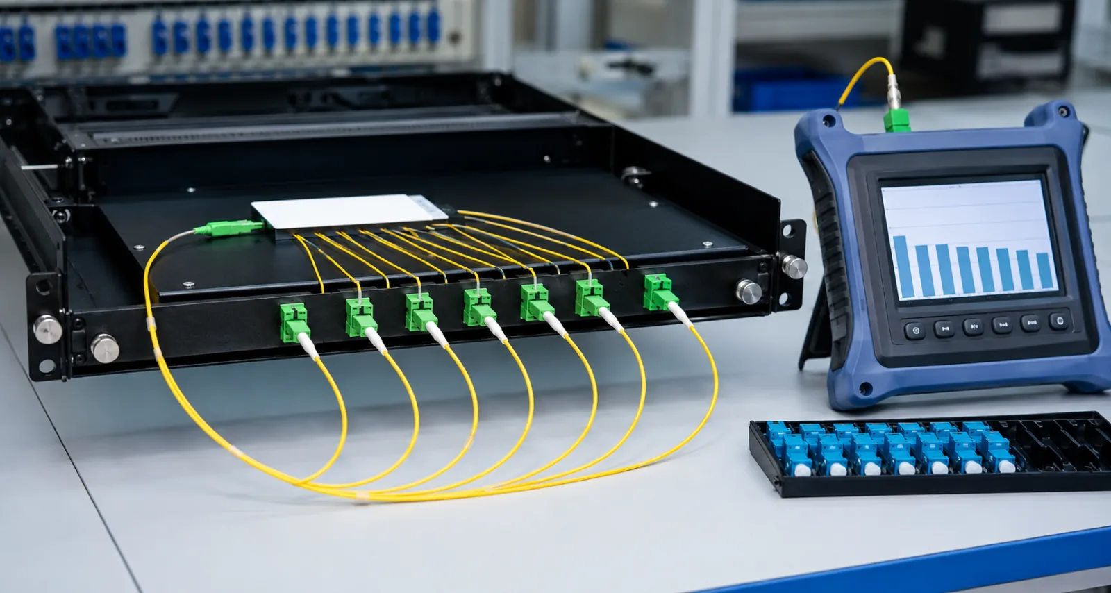
Summary: Useful PLC splitter uniformity acceptance criteria must distinguish three quantities: each path’s insertion loss, the spread between output paths, and loss beyond the ideal split. Test every required port at every specified wavelength, preserve raw readings and apply the agreed standard rather than accepting an attractive average.
The worked table below is hypothetical. It demonstrates calculations and is not a factory test report, product certificate or guaranteed Liqiba specification.
Three loss terms that buyers should separate
Insertion loss is the loss from a stated input to a stated output. It includes the power division and component losses under the measurement reference.
Uniformity describes the spread among output path losses. For a defined set, calculate maximum measured insertion loss minus minimum measured insertion loss. Lower spread means outputs are more closely balanced.
Excess loss compares measured behavior with ideal power division. For a symmetrical 1×N splitter, ideal splitting loss is 10 log10(N). This theoretical number is not a purchase limit because real components and connections add loss.
ITU-T G.671 specifies transmission characteristics for optical branching components, including insertion loss, reflectance, directivity and uniformity. ITU-T G.9940 gives a practical system example with splitter insertion loss and channel-uniformity values. Project requirements may use other relevant IEC or operator specifications, so name the governing document and edition.
Build the table before testing
Define splitter type, input used, output count, connectorization, operating wavelengths, direction, reference method, test equipment and environmental condition. A bare 1×8 device and a connectorized module do not have identical measurement boundaries.
Create one row for every output at every wavelength. Include equipment serial number, calibration status, reference cord identity and timestamp. Do not record only “pass” because the raw values are needed to audit uniformity.
Worked 1×8 example
Assume a connectorized symmetrical 1×8 splitter measured from input to each output at 1310 nm. Assume the project maximum insertion loss is 10.5 dB and maximum uniformity is 1.0 dB. These example limits mirror values shown for a particular 1×8 system example in ITU-T G.9940; they are not universal product claims.
| Output | Measured insertion loss | Against 10.5 dB path limit |
|---|---|---|
| 1 | 9.72 dB | Pass |
| 2 | 9.88 dB | Pass |
| 3 | 10.04 dB | Pass |
| 4 | 9.79 dB | Pass |
| 5 | 10.18 dB | Pass |
| 6 | 9.94 dB | Pass |
| 7 | 10.31 dB | Pass |
| 8 | 9.85 dB | Pass |
Worst insertion loss is 10.31 dB. Best insertion loss is 9.72 dB. Uniformity is therefore 10.31 − 9.72 = 0.59 dB, which passes the assumed 1.0 dB limit. All individual outputs also pass the assumed 10.5 dB limit.
Calculate theoretical and excess loss carefully
Ideal loss for 1×8 is 10 log10(8) = 9.03 dB. If a team uses the worst path for a conservative comparison, its apparent excess above ideal is 10.31 − 9.03 = 1.28 dB. If it uses the arithmetic average of the eight example path losses, 9.96 dB, the average excess is about 0.93 dB.
Those two values answer different questions. State the convention. Connector loss and the reference plane can be embedded in measured insertion loss, so do not compare an unconnectorized chip specification with a connectorized-module measurement without adjustment.
Why an average can hide a failure
Imagine output 7 were 10.72 dB while the other values remained the same. The average could still appear reasonable, but output 7 would fail a 10.5 dB per-path limit. Uniformity would also become 1.00 dB using the displayed precision, right at the assumed boundary.
Retain adequate measurement resolution and apply the contract’s rounding rule. Do not round a 10.54 dB raw value to 10.5 dB unless the governing procedure explicitly permits it. Measurement uncertainty also needs an agreed decision rule near a limit.
Keep wavelength sets independent
Stabilize the source and allow equipment to warm up as specified. Establish the reference without disturbing connections that the method expects to remain fixed. If a reference cord is disconnected, determine whether the reference must be repeated. A drifting source or changing reference can create a false pattern across sequential ports.
Randomize or repeat a subset of port measurements when diagnosing a suspicious monotonic trend. If later ports all appear worse, the cause may be source drift, contamination or cord movement rather than splitter uniformity. A repeated port provides a simple stability check, although the governing procedure should define formal requirements.
Repeat the complete table at every specified wavelength, often including 1310 nm and 1550 nm and any maintenance or service band required by the project. Use wavelength-appropriate references and stable launch conditions.
A label such as “uniformity 0.6 dB” is incomplete without wavelength, direction, ports included and measurement boundary. If one output is excluded due to damage, report that exclusion; do not silently calculate uniformity on the remaining ports.
Inspect the physical configuration
Confirm connector polish, adapter condition, fiber type, package, lead length and port labeling. Inspect and clean both sides before mating. A contaminated reference connection can create an apparent high-loss port and contaminate subsequent interfaces.
For unconnectorized devices, define the splice or temporary coupling method. For modules, distinguish component loss from field connector loss if the contract requires separate limits. Never mix APC and UPC interfaces.
Turn data into a procurement decision
Define lot sampling separately from numerical acceptance. Testing all ports on one sampled device does not establish the behavior of every device in a shipment. The purchase plan should state sample size, lot identity, treatment of failures and whether supplier test data are required for each serialised unit.
When a retest follows cleaning, retain both readings and the reason for retest. Do not overwrite the first result. If the retest passes, the record should show whether contamination was confirmed, whether the reference was re-established and which value governs disposition under the agreed procedure.
| Acceptance item | Required record | Failure response |
|---|---|---|
| Every path loss | Input, output, wavelength and dB | Retest after controlled interface check |
| Uniformity | Max, min and subtraction | Identify outlier and product disposition |
| Reflectance/directivity if specified | Method and result | Apply governing component criteria |
| Traceability | Lot, serial, equipment and file | Hold material until reconciled |
The commercial PLC splitter manufacturer page is the appropriate place to request split ratio, package, connectorization and project documentation. Put numerical limits and test boundaries in the inquiry rather than asking only for “low loss.”
Our FTTH 1×32 splitter loss-budget guide explains system budgeting, while the cascaded-splitter worksheet shows why worst-case losses must be added through multiple stages. Component acceptance and network budgeting are related but separate decisions.
Issue a reproducible acceptance record
Photograph the port labels and module identity when the quality plan permits it, but do not treat a photograph as a substitute for the measurement file. Link both artifacts with the same sample identifier.
When results are transferred into a spreadsheet, protect formulas and retain a read-only raw-data export. Manually retyping dozens of port values creates avoidable transcription and sorting errors.
Check labeling against the measured port map. A numerically acceptable module can still be unusable if pigtails or adapter positions are misidentified. For 2×N devices, identify which input was used and whether both inputs require testing; do not collapse two input matrices into one “typical” value.
Also preserve units and sign conventions. Splitter insertion loss is normally recorded as a positive loss value, while an instrument may display relative power with a negative sign. Normalize the report deliberately and keep the raw export so a sign conversion cannot create an apparent gain or false failure.
A final record should contain the approved specification, product configuration, measurement reference, all port values, calculations, uncertainty decision rule and disposition. A screenshot of one favorable port is not adequate evidence for an eight-, sixteen- or thirty-two-output device.
The core rule is simple: individual path compliance prevents a weak output from hiding in an average, while uniformity controls balance across the set. Keeping both checks makes the purchase decision technically meaningful.
Frequently Asked Questions
Is splitter uniformity the same as insertion loss?
No. Insertion loss describes loss through an individual path. Uniformity is the difference between the highest and lowest path loss within the defined test set and wavelength.
Can I accept a splitter using average insertion loss?
Not if the specification limits every output. An acceptable average can conceal one failing port, so retain and compare each measured path.
Is theoretical splitting loss the procurement limit?
No. The ideal value excludes excess loss and connection effects. Use the agreed component standard, product specification and test reference method.
Should 1310 nm and 1550 nm results be combined?
Keep them separate unless the approved specification explicitly defines a combined calculation. A port can behave differently by wavelength.
Does this worked 1×8 table represent Liqiba production data?
No. It is a hypothetical calculation example showing the method. Product acceptance requires actual, traceable measurements and agreed limits.