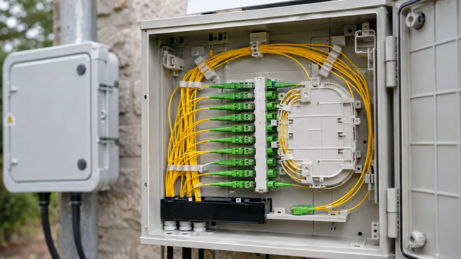
Scope: This worksheet compares passive branch layouts for planning and procurement. It is not a declaration that a particular splitter assembly meets a PON optical class. Before ordering, the project engineer must reconcile every branch with the selected OLT and ONT specifications, including operating wavelengths and minimum as well as maximum permitted path loss. Keep component revisions and connection boundaries beside the calculation so a substitution can be assessed without rebuilding the model from memory.
Summary: A cascaded 1×4 and 1×8 splitter loss budget follows one subscriber path through two devices. It does not add the losses of every splitter in the neighborhood. The ideal division is equivalent to 1:32, while the real result depends on device excess loss, joints, fiber length and the required operating reserve. This worksheet compares that path with a centralized 1×32 design.
The choice has consequences beyond attenuation. Splitter location changes distribution-fiber demand, access for repairs, subscriber assignment and the amount of infrastructure exposed during maintenance. Complete the optical calculation and the operating comparison before selecting the topology.
Draw the tree and identify one path
In the example cascade, one feeder enters a 1×4 device. Each of its four outputs can feed a separate 1×8 device. Each second-stage device serves up to eight final outputs. Full population therefore requires four second-stage devices, although an individual subscriber signal passes through only one of them.
CommScope’s centralized architecture explanation describes the distinction between concentrating splitters at a hub and distributing stages across the network. Centralization simplifies access and allocation; cascading can reduce fiber requirements on selected distribution sections while adding management complexity.
Label the path explicitly: OLT port, feeder fiber, first-stage input and output, interstage fiber, second-stage input and output, drop and ONT. Attach lengths and component identities to that chain. This prevents the common mistake of summing every box shown on the network drawing.
Understand ideal loss without treating it as a product limit
For equal power division among N outputs, ideal positive attenuation per output is 10 log10(N) dB. Thus a 1×4 contributes about 6.02 dB and a 1×8 about 9.03 dB. Their sum is 15.05 dB, the same ideal result as 10 log10(32).
Actual devices include excess loss and port variation. The FOA passive-device testing guide explains why splitter acceptance records must cover individual outputs rather than relying on split ratio alone. Use guaranteed maximum values at the required wavelengths and conditions for design; a favorable typical value is not a bound on every output.
Worked comparison with explicit component boundaries
Assume two hypothetical alternatives serving a subscriber over 10 km of total fiber. For both, use 0.35 dB/km attenuation, four external mated connections at 0.30 dB each, eight external splices at 0.10 dB each and 3.0 dB reserve. Assume a centralized splitter assembly rated at 17.0 dB maximum insertion loss.
For the cascade, assume first-stage and second-stage assemblies rated at 7.2 and 10.5 dB. Their stated values already include the supplier-defined device termination losses. Add only one further 0.30 dB interstage connection outside those boundaries. These assumptions are deliberately explicit to prevent connector double counting; they are not Liqiba product specifications.
| Loss item | Single 1×32 | 1×4 plus 1×8 path |
|---|---|---|
| Specified splitter assemblies | 17.0 dB | 7.2 + 10.5 = 17.7 dB |
| Total fiber | 10 × 0.35 = 3.5 dB | 3.5 dB |
| Four external connections | 1.2 dB | 1.2 dB |
| Eight external splices | 0.8 dB | 0.8 dB |
| Additional interstage connection | 0 dB | 0.3 dB |
| Physical path allowance | 22.5 dB | 23.5 dB |
| Planning reserve | 3.0 dB | 3.0 dB |
| Total required budget | 25.5 dB | 26.5 dB |
If a fictional equipment specification allowed a 28.0 dB maximum budget under the relevant conditions, the remaining allowance after reserve would be 2.5 dB centrally and 1.5 dB for the cascade. The 28.0 dB figure is an example assumption, not a claim that all PON equipment supports that budget.
Check the longest branch and the shortest branch
If one cascade branch adds 2 km and two further 0.10 dB splices, its required budget increases by 0.7 + 0.2 = 0.9 dB. The remaining allowance falls from 1.5 to 0.6 dB. This sensitivity check shows why an average route length is insufficient for acceptance planning.
The shortest branch needs a separate minimum-loss check against receiver overload and the equipment’s permitted optical distribution network range. A 3 dB reserve is not a physical attenuator and must not be included as real loss in that calculation. Repeat the budget for the opposite transmission direction and relevant wavelength band.
Compare the operating model
| Question | Centralized design | Cascaded design |
|---|---|---|
| Where are splitter ports assigned? | Primarily at one hub | Across hub and field-stage locations |
| What must the inventory track? | Hub splitter and output | First-stage output plus second-stage device and output |
| What can constrain expansion? | Hub capacity and distribution fibers | Branch allocation and field enclosure capacity |
| What complicates troubleshooting? | Access to the centralized hub | Multiple passive stages and shared trace interpretation |
Evaluate a partially occupied neighborhood as well as the final build. An unused second-stage port still receives its designed share; passive splitting does not automatically shift that power to active subscribers. Consider the truck visits, splice work and access needed when a new customer is connected later.
What to request from a splitter supplier
Specify split ratio, input count, wavelength range, connector or bare-fiber format, maximum insertion loss, output uniformity and enclosure requirements. Ask whether connector losses are included and under what reference method. Request output-level records that can be linked to a device serial number or other traceable identifier.
The PLC splitter manufacturer page is the commercial destination for that specification. The PLC splitter selection guide supplies broader background, and the FTTH network design guide connects the component decision to the access architecture.
Use a branch register for expansion and troubleshooting
Create one record per subscriber output. Include the first-stage device and port, second-stage device and port, feeder section, interstage section, drop length and termination locations. Associate each record with its own loss limit. This makes the network manageable when two streets have different distances or when one enclosure contains an additional connection.
For a staged deployment, mark outputs as active, reserved, unassigned or unavailable. A reserved output may be committed to a future building even though it has no present traffic. Keep that status separate from the optical state of the port so a technician does not accidentally allocate it to another subscriber.
Review a second-stage replacement
If a replacement 1×8 device has a maximum specified loss 0.4 dB higher than the original, every path using that device needs the additional 0.4 dB reviewed. The effect is local to that branch group, not automatically the entire network. Update the register, retain the old component record and retest the affected paths under the agreed procedure.
A connectorized replacement may also change the measurement boundary. Compare the complete assembly definition rather than subtracting two headline splitter values. A lower device-only loss can be offset by additional external joints, while a quoted assembly value may already include them.
Check service evolution explicitly
Adding a coexistence filter or changing the PON technology can introduce new wavelength-dependent losses and operating constraints. Reuse the branch inventory, but rebuild the optical checks using the new interface data. The unchanged numerical split ratio is not evidence that the upgraded system has the same permitted path range.
Include field access in the decision as well. A component with a small optical advantage may create longer restoration times if its enclosure is difficult to reach. The useful architecture comparison combines branch margin, port allocation, access work and the actual service plan.
Acceptance records should reproduce the path
For every final output, retain the complete stage-to-stage mapping, operating wavelengths, fiber lengths, loss limits and actual measurements. Record test direction and reference method. Device acceptance and installed-network acceptance are separate records; a passed factory component cannot prove the completed route meets its budget.
When a branch fails, compare the measured path with its own worksheet and component records. Check connectors, port identity and unexpected joints before changing the topology. A good handover lets the next engineer reproduce the calculation from the labeled path without reconstructing the whole deployment from memory.
Frequently Asked Questions
Does a 1×4 followed by a 1×8 produce a 1:32 split?
For an equally split fully populated arrangement, yes: four first-stage outputs can feed four separate eight-output second stages, providing 32 final outputs. A subscriber path traverses one 1×4 and one 1×8.
Should all second-stage splitters be added to one subscriber budget?
No. Add only the components on that subscriber path. The other second-stage devices belong to different branches and do not contribute their individual insertion losses in series to this path.
Is cascaded splitting always lossier than a single splitter?
Not as a universal rule. Ideal splitting loss is the same for the same total equal split. Real component limits, additional joints and measurement boundaries determine the practical difference.
Can a spare output increase the power available to active outputs?
Not for a conventional fixed equal-ratio passive splitter. An unused output does not redistribute its share to the active ports. Keep it protected and include the device full split ratio in the budget.
Does passing this worksheet prove GPON or XGS-PON compatibility?
No. Verify the selected OLT and ONT optical classes, both wavelength directions, minimum and maximum path loss, differential reach, protocol requirements and any coexistence components.